Introduction
The objective of this project was to use Matlab and Simulink to model, simulate, and control a two-wheeled robot based on the Lego Mindstorms EV3 system. The project allowed us to explore several control techniques, including proportional control, proportional-integral control, and state feedback control to stabilize the system.
Robot Parameters
The two-wheeled robot was modeled based on the following parameters:
- Physical Constants:
- Gravity acceleration : g=9.81m/s2
-
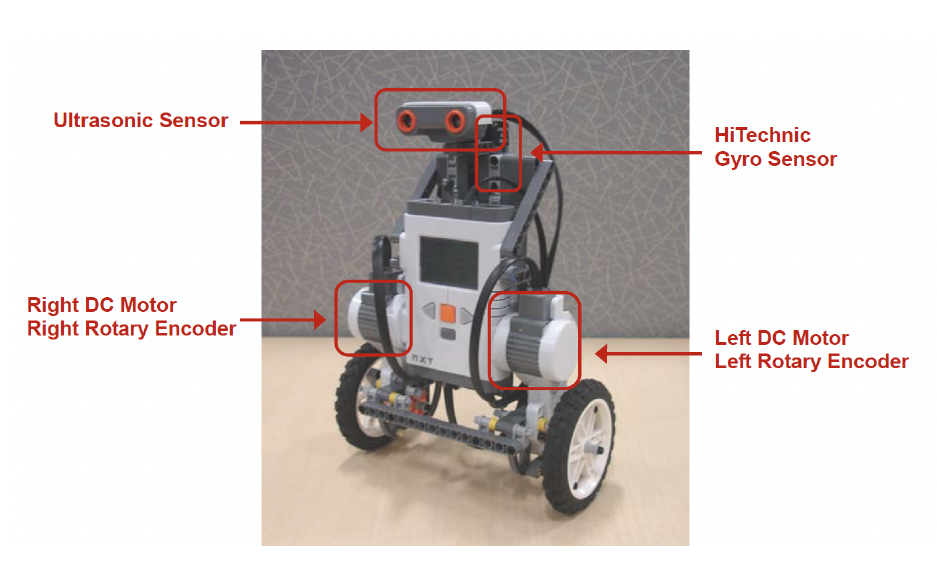
Lego Mindstorms Parameters:
-
Wheel weight 𝑚=0.03kg
-
Wheel radius 𝑅=0.042m
-
Body weight 𝑀=0.67kg
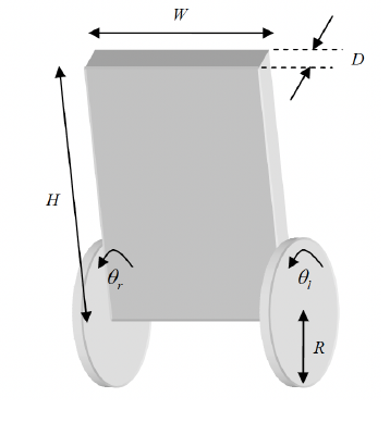
-
Body width 𝑊=0.165m
-
Body height 𝐻=0.152m
-
Center of mass distance 𝐿=𝐻/2
-
Friction coefficients 𝑓𝑚=0.0022 = 𝑓𝑤=0
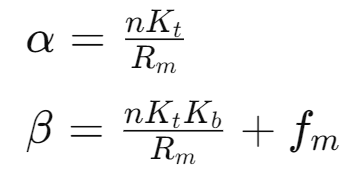
-
From these parameters, we calculated the constants used in the system dynamics:
Process Modeling
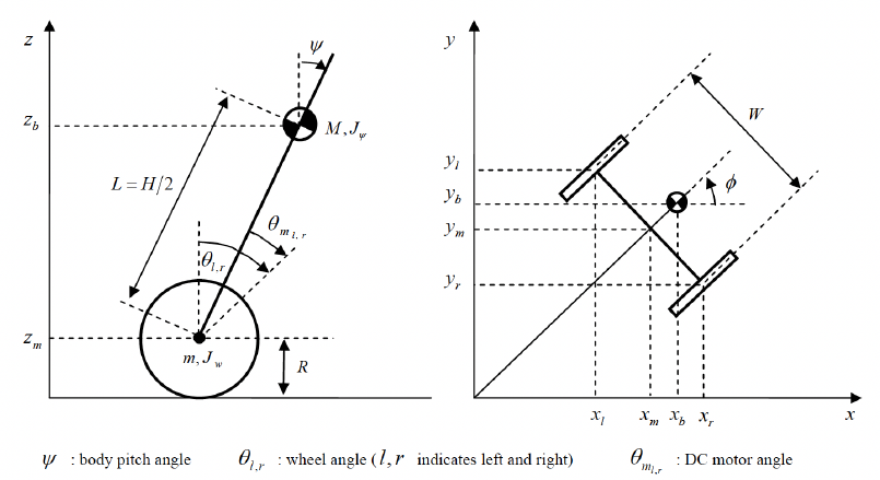
MIMO State-Space Models
The system’s state-space representation was derived by modeling the robot’s motion using the Lagrangian method. The following matrices define the system:
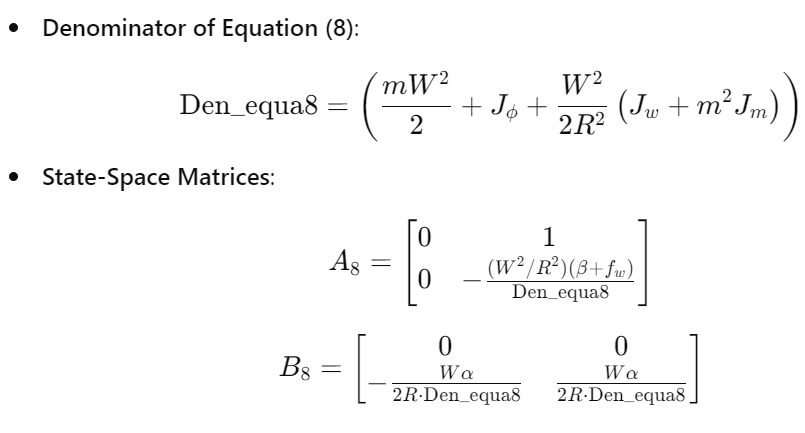
SISO State-Space Model
We reduced the MIMO model to a SISO state-space model for balance control, simplifying the input to 𝑢=(𝑣𝑙+𝑣𝑟)/2. The resulting system was defined as: sys = ss(A, B, C, 0)
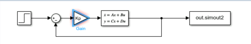
Simulation of the System with Simulink
We first tested the open-loop response of the system to a step input of 1V. Below is the code used for plotting the system’s response:
sim("Simulink1.slx")
plot(out.simout.Time, out.simout.Data);
xlabel('Time(s)');
ylabel('Theta(°)');
title('Response to a Step Input');
Next, we tested the system’s response to an impulse input. In both cases, the system was unstable, as the signal did not stabilize and continued increasing without bound.
Open-Loop Analysis
We analyzed the system for observability and controllability. Both matrices’ ranks were equal to the rank of matrix 𝐴, confirming that the system is observable and controllable:
rank(obsv(sys))  % Observability rank
rank(ctrb(sys))  % Controllability rank
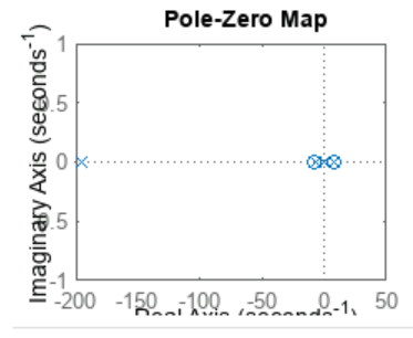
The system was found to be unstable, as shown by the pole-zero map and damping analysis:
figure; pzmap(sys);
figure; damp(sys);
isstable(sys);
Control System Design
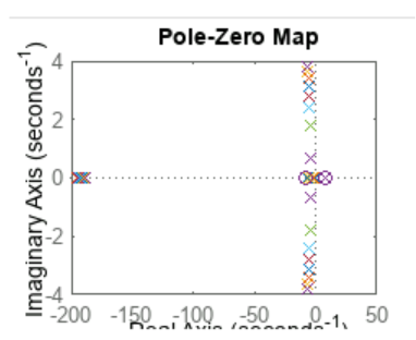
Proportional Control
We implemented a proportional controller to stabilize the system. Despite varying the gain 𝐾𝑝, the system remained unstable:
for Kp = 0.1:1:10.1
    pzmap(feedback(TransferFunction*Kp, 1));
    hold on;
end
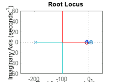
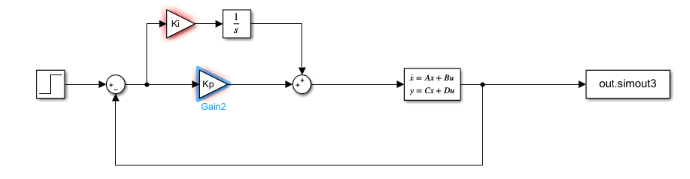
Proportional-Integral Control
Next, we implemented a proportional-integral (PI) controller. However, the system remained unstable for any combination of 𝐾𝑝 and 𝐾𝑖, as the Routh table analysis showed that there were always positive terms in the first column:
syms Kp Ki EPS
routh([1 193 127*Kp-265 14*Kp+127*Ki-9109 -8875*Kp+14*Ki -8875*Ki], EPS)
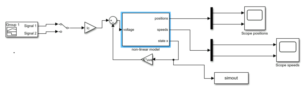
State Feedback Control
Finally, we implemented a state feedback controller, which successfully stabilized the system. However, the control signal exhibited significant error, which we corrected by adding a pre-gain 𝑙𝑐.
step_value = pi/5;
lc = step_value / (-0.03);
sim('Simulink2.slx');
plot(out.simout4.Time, out.simout4.Data);
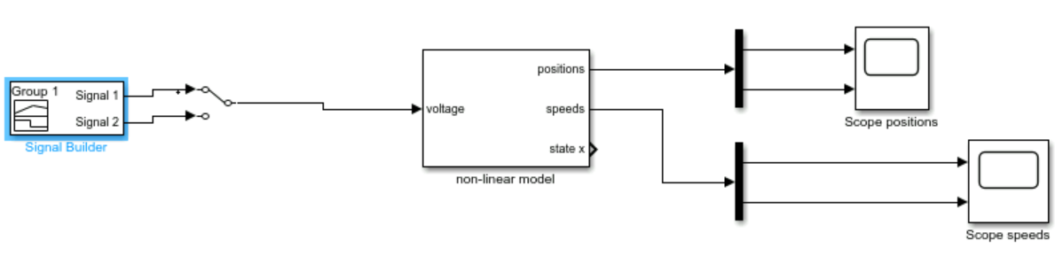
Nonlinear Simulations
Using the provided NXTwaySim Simulink file, we performed nonlinear simulations to validate the control laws. Without feedback, the system was unstable, but with state feedback, the robot maintained balance:
play_animation(positions1, simtime1);
Conclusion
This project allowed us to explore and apply various control techniques to a complex, real-world system using Matlab and Simulink. While proportional and PI controllers did not provide the necessary stability, the state feedback controller proved to be an effective solution. The project highlighted the importance of state feedback in stabilizing systems where simpler control strategies fail.
The project also provided valuable experience in modeling and simulating control systems and deepened our understanding of the theoretical concepts covered in class